Lensa ML

How Regularization Works

Step 1 of 6: The Overfitting Problem

When the model memorizes instead of learning

xyGood fit
TrainTest
Train Loss
0.125
Test Loss
0.013

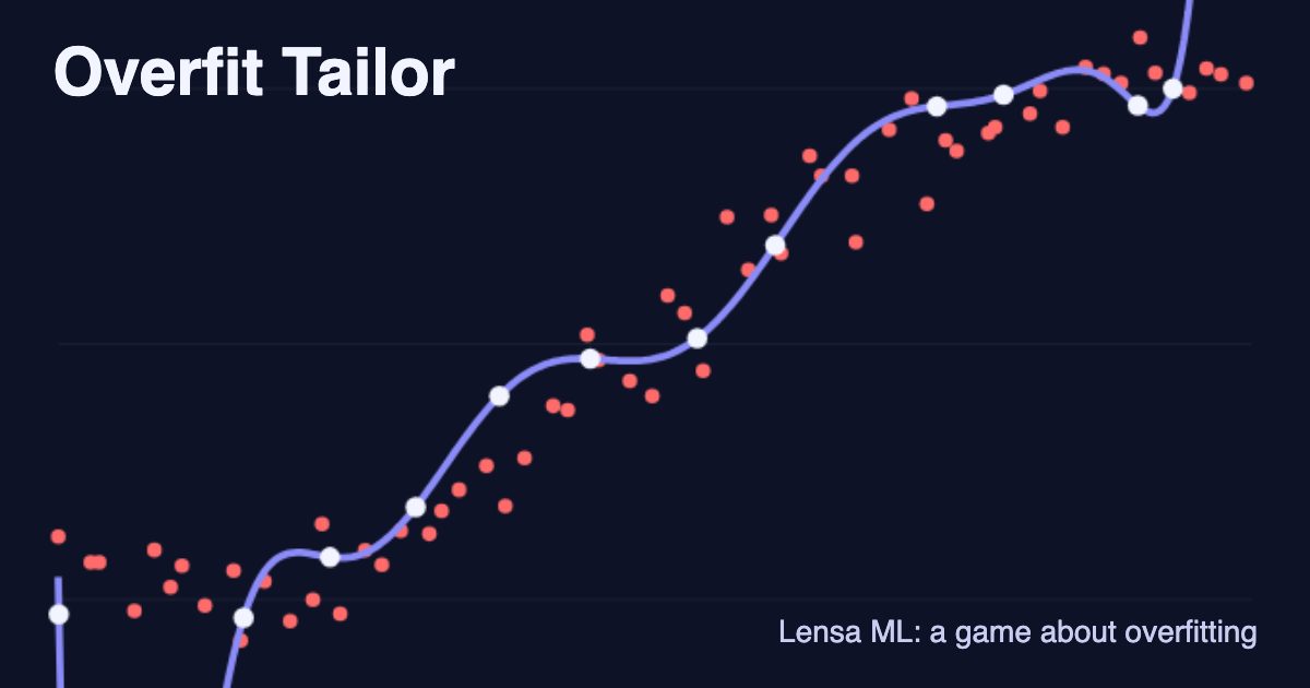
An overfit model memorizes training noise: its training loss is tiny, but it fails on new data. A good fit captures the true pattern and generalizes.

Press Show Overfit and compare the two loss cards. The overfit curve is a sum of 18 narrow bumps, one centered on each training point, with weights solved so the curve hits every point exactly. Its train loss is essentially zero, and its test loss on the 5 held-out points is about 0.19, against 0.013 for the true curve y = 0.5x². Any model with one free parameter per data point can do this. Regularization keeps the same flexible model but makes extreme weights expensive.

Step 2 of 6: L2 Regularization

Penalizing large weights to keep things smooth

λ = 0.00
TrainTestTrue f(x)
No regularizationλ = 0.00Strong
Train Loss
0.000
Test Loss
0.188
λΣw²
0.00
Weight magnitudes |wᵢ| (Σw² = 2691k) · ^ = off scale
0.002.04.0

With λ ≈ 0, there is no regularization. Weights are huge and varied, so the curve wiggles through every point. Train loss is near zero but test loss is high.

Drag λ from 0 to 5 and watch Σw² in the bar chart title. Without a penalty, Σw² is in the millions, because huge positive and negative weights cancel to thread the curve through every point. At λ = 1 it falls to about 2.3. L2 adds λΣw² to the loss, so each gradient step also pulls every weight toward zero in proportion to its size. That is why L2 is often called weight decay. In linear regression the same penalty is called ridge regression.

Step 3 of 6: L1 Regularization

Pushing weights to exactly zero — built-in feature selection

L1 λ = 0.00
TrainTestTrue f(x)
No regularizationλ = 0.00Strong
Train Loss
0.028
Test Loss
0.143
λΣ|w|
0.00
Zeros
0/18
Weight magnitudes |wᵢ| (Σw² = 10.7)
0.001.12.2

With λ ≈ 0, there is no regularization. All weights are active and the model overfits the noisy training data.

Drag λ and count the red bars, which mark weights set to exactly zero. L1 adds λΣ|w|, whose gradient has the same size, λ, for every nonzero weight. A small weight gets pushed just as hard as a large one, so it reaches zero and stays there. The solver here uses soft thresholding: after each gradient step, w becomes sign(w)·max(|w| − η·λ, 0). At λ = 1, 13 of the 18 weights are zero. In linear regression this penalty is called the lasso.

Step 4 of 6: Dropout

Randomly silencing neurons during training

×××InputHidden 1Hidden 2Output
Rate
40%
Effective weights: 6/9 neurons active
0.000.941.9

Dropout randomly silences neurons each training step, so the network cannot rely on any single path. The weight chart shows how dropped neurons have their effective weight zeroed out. At test time all neurons are active, with outputs rescaled to match. Currently dropping 3 of 9 hidden neurons.

Toggle dropout and move the rate slider between 10% and 80%. This network has 9 hidden neurons, so dropout samples from 2^9 = 512 possible subnetworks, and training averages over them. Most frameworks use inverted dropout. During training they divide the surviving activations by (1 − p), so at test time the full network runs unchanged. Typical rates are 0.5 for large fully connected layers and around 0.1 in transformers. Srivastava et al. (2014) introduced the method.

Step 5 of 6: Early Stopping

Stop training before overfitting kicks in

EpochLossoverfit zonelearningepoch 28
Train lossVal loss
Epoch 0Epoch 0Epoch 60
Train Loss
2.050
Val Loss
2.150
Gap
0.100
‖w‖
0.50

Training hasn't progressed much yet. Both train and val loss are still high. Press Play or drag the slider. These curves are an illustrative sketch of a typical run, not the output of a real training run.

Press Play, or drag the epoch slider, and watch where the validation curve turns up. In this run the best validation loss comes at epoch 28 of 60. In practice, training code saves a checkpoint whenever validation loss improves. It stops after a set number of epochs without improvement, called the patience, and restores the best checkpoint. Early stopping limits how far the weights travel from their small initial values. For linear models, Goodfellow et al. show that it behaves much like an L2 penalty.

Step 6 of 6: Comparison

How each technique shapes the fit

No Reg
Method
Train Loss
Test Loss
No Reg
0.000
0.188
L2
0.072
0.062
L1
0.127
0.073
Dropout (≈L2)
0.051
0.105
Early Stop
0.115
0.026
True f(x)
0.125
0.013
All losses are MSE computed on the same 18 train / 5 test points from Step 1. L2: ridge fit on the RBF features with λ=1. L1: ISTA solver with λ=1. Dropout: approximated as L2 with λ=0.5 (dropout ≈ implicit L2). Early stop: gradient descent from zero weights, halted at 40 iterations.

No Reg: Overfits by memorizing noise. Train loss is near zero but test loss is high, the classic sign of overfitting.

Click each method and compare its row in the loss table. Early stopping at 40 iterations and L2 with λ = 1 give the lowest test losses of the regularized fits, about 0.026 and 0.062, against 0.188 with no regularization. Run the same gradient descent for 400 iterations and its test loss climbs back to about 0.18. The best λ, dropout rate, or stopping point always depends on the data, so these settings are tuned on a validation set. Real training runs usually combine several methods, for example weight decay plus dropout plus early stopping, along with data augmentation.

What is regularization in machine learning?

Regularization is any technique that reduces overfitting by limiting how closely a model can fit its training data. The most common form adds a penalty on the size of the weights to the loss: L_total = L_data + λ·R(w), where λ sets the strength. Other forms change the training procedure instead, such as dropout and early stopping.

Almost every trained model uses some regularization. Ridge and lasso regression add L2 and L1 penalties to linear models. Deep networks typically combine weight decay, dropout, data augmentation, and early stopping. Large language models are trained with AdamW, whose decoupled weight decay is a form of L2 regularization, and many use dropout during fine-tuning.

Key ideas

  • Regularization trades a little training accuracy for better performance on new data.
  • L2 regularization shrinks all weights in proportion to their size.
  • L1 regularization drives small weights to exactly zero and produces sparse models.
  • Dropout randomly disables neurons during training so no unit can depend on another.
  • Early stopping halts training when validation loss stops improving.
  • The regularization strength is a hyperparameter chosen with validation data.

Short takes on this topic

Common questions

What is the difference between L1 and L2 regularization?

L1 penalizes the sum of absolute weights and tends to set many weights to exactly zero, which acts as feature selection. L2 penalizes the sum of squared weights and shrinks all of them smoothly without making them zero. Elastic net combines both penalties.

Is weight decay the same as L2 regularization?

For plain gradient descent, yes: adding λΣw² to the loss is equivalent to shrinking each weight by a constant factor every step. For adaptive optimizers such as Adam, the two differ, because Adam rescales the penalty's gradient per weight. AdamW applies the decay directly to the weights, which usually works better.

How do I choose the regularization strength λ?

Try values on a logarithmic grid, such as 0.0001, 0.001, 0.01, and 0.1, and keep the one with the best validation score. Cross-validation gives a more reliable choice when data is limited. If validation error is high and close to training error, λ is probably too large.

Is data augmentation a form of regularization?

Yes. Flipping, cropping, or adding noise to training examples creates new variations of the data, which makes memorization harder. It changes the data rather than the loss or the model, and it is one of the most effective regularizers for image and audio models.

Related explainers

References

  1. Srivastava et al. (2014), "Dropout: A Simple Way to Prevent Neural Networks from Overfitting", JMLR
  2. Loshchilov & Hutter (2017), "Decoupled Weight Decay Regularization"
  3. Goodfellow, Bengio & Courville (2016), "Deep Learning", chapter 7: Regularization for Deep Learning
  4. James, Witten, Hastie & Tibshirani, "An Introduction to Statistical Learning", chapter 6: ridge regression and the lasso

Last updated